Lecture 22 - Diffusion Models for Text-to-Image Generation

![]()
22.1 Generative Text-to-Image Models
Generative models are a category of Machine Learning models that generate new data instances, typically based on the learned data distribution of the training dataset. This is different from most models that we studied so far, such as discriminative models that can be used to classify data instances into several classes, for example.
The family of GAN models (StyleGAN, CycleGAN, BigGAN, etc.) have been the most important category of generative models since the original GAN paper was published in 2014. Despite the remarkable progress in image synthesis achieved by the family of GAN models, these models are generally difficult to train due to their adversarial nature, as well as there is a lack of diversity in generated images.
Another group of generative models were recently been introduced, referred to as Denoising Diffusion Probabilistic Models (DDPMs), or they are also simply called Diffusion Models. Diffusion Models convert Gaussian random noise into images from a learned data distribution in an iterative denoising process. This approach is inspired by the physical process of gas diffusion, and has also applications in other scientific fields. Diffusion Models have demonstrated an ability to generate images with increased quality and diversity in comparison to GANs, and they don’t suffer from mode collapse and other training instabilities that are characteristical for GANs.
Examples of recent text-to-image generative methods that are based on Diffusion Models include DALL-E 2 by OpenAI, Stable Diffusion by Stability.AI, and ImageGen by Google Brain.
Text-to-image generative models rely on learned representations by Large Language Models that are trained on pairs of images and image captions. These representations are afterward used to guide a Diffusion Model in generating new images given a text prompt.
This group of generative models can also take an input image as a prompt, and generate an image similar to the input image. For instance, we can quickly draw a simple drawing manually, and use it to create a photorealistic image.
22.2 High-Level API for Stable Diffusion with Keras
Let’s first show an example of a high-level API for generating images from text prompts, and afterward we will explain the components in text-to-image models.
The code in the next cells employs a Keras library for Computer Vision called keras_cv that implements the Stable Diffusion model. Stable Diffusion was the first text-to-image model that was open-sourced, and this motivated a large number of recent applications.
To run the model we need to first install the keras_cv package. Afterward, we can just load a Stable Diffusion model and give a prompt to generate images.
[ ]:
!pip install keras_cv --upgrade --quiet
     ━━━━━━━━━━━━━━━━━━━━━━━━━━━━━━━━━━━━━━━━ 803.1/803.1 kB 10.8 MB/s eta 0:00:00
     ━━━━━━━━━━━━━━━━━━━━━━━━━━━━━━━━━━━━━━━━ 950.8/950.8 kB 48.5 MB/s eta 0:00:00
[ ]:
import keras_cv
from tensorflow import keras
import matplotlib.pyplot as plt
Using TensorFlow backend
[ ]:
# instantiate a Stable Diffusion model
model = keras_cv.models.StableDiffusion(img_width=512, img_height=512)
By using this model checkpoint, you acknowledge that its usage is subject to the terms of the CreativeML Open RAIL-M license at https://raw.githubusercontent.com/CompVis/stable-diffusion/main/LICENSE
[ ]:
# generate images (it takes a few minutes with Google Colab Pro)
images = model.text_to_image("photograph of an astronaut riding a horse", batch_size=3)

# plot the images
plt.figure(figsize=(16, 8))
for i in range(len(images)):
    ax = plt.subplot(1, len(images), i + 1)
    plt.imshow(images[i])
    plt.axis("off")
Downloading data from https://github.com/openai/CLIP/blob/main/clip/bpe_simple_vocab_16e6.txt.gz?raw=true
1356917/1356917 [==============================] - 0s 0us/step
Downloading data from https://huggingface.co/fchollet/stable-diffusion/resolve/main/kcv_encoder.h5
492466864/492466864 [==============================] - 2s 0us/step
Downloading data from https://huggingface.co/fchollet/stable-diffusion/resolve/main/kcv_diffusion_model.h5
3439090152/3439090152 [==============================] - 14s 0us/step
50/50 [==============================] - 176s 2s/step
Downloading data from https://huggingface.co/fchollet/stable-diffusion/resolve/main/kcv_decoder.h5
198180272/198180272 [==============================] - 4s 0us/step

[ ]:
# generate images (it takes a few minutes per image with Google Colab Pro)
images = model.text_to_image("ruins of an ancient castle in a desert, concept art", batch_size=3)

# plot the images
plt.figure(figsize=(16, 8))
for i in range(len(images)):
    ax = plt.subplot(1, len(images), i + 1)
    plt.imshow(images[i])
    plt.axis("off")
50/50 [==============================] - 95s 2s/step

[ ]:
# generate images
images = model.text_to_image("a cute magical flying dog, fantasy art, golden color, high quality, highly detailed, elegant, sharp focus,"
    "concept art, character concepts, digital painting, mystery, adventure",  batch_size=3)

# plot the images
plt.figure(figsize=(16, 8))
for i in range(len(images)):
    ax = plt.subplot(1, len(images), i + 1)
    plt.imshow(images[i])
    plt.axis("off")
50/50 [==============================] - 95s 2s/step

22.3 Denoising Diffusion Probabilistic Models
Denoising diffusion probabilistic process consists of two phases:
Forward diffusion process, in which Gaussian noise is gradually added to an image, until the image becomes complete random noise.
Reverse diffusion process, in which the image with Gaussian noise is gradually denoised, until all noise is removed and the original image is recovered.
22.3.1 Forward Diffusion Process
For an initial image denoted \({x}_0\) that is sampled from the data distribution \(q(x)\), the forward diffusion process adds noise over \(T\) consecutive steps. At each step, the added Gaussian noise has variance \(\beta_{t}\). I.e., the sample \({x}_{t}\) that corresponds to step \(t\) of the forward process is obtained by adding Gaussian noise to the sample \({x}_{t-1}\) from step \(t−1\). Therefore the conditional probability density of the forward diffusion process \(q({x}_t |{x}_{t-1})\) can be written as:
The above notation means that \({x}_t\) has Gaussian distribution, with a mean \(\sqrt{1-\beta_{t}}{x}_{t-1}\) and variance \(\beta_{t}\mathbf{I}\).
This process is depicted in the next figure.

Figure: Forward diffusion process.
Such process where the probability of an event at any given state is dependent only on the immediately preceding state is called Markov Chain or Markov Process.
The mean and variance of the samples depend on a parameter \(\beta_{t}\), which defines the level of added Gaussian noise. The value of \(\beta_{t}\) can either be constant for all steps, or it can be gradually changed (e.g., by using a sigmoid, cosine, tanh, linear function, etc).
Substituting \(\alpha_{t}=1-\beta_{t}\), and \(\bar{\alpha}_{t} = \prod_{s=1}^{t} \alpha_{s}\), the distribution can also be rewritten as:
This substitution allows to draw samples at any timestep by using only the initial image \(x_0\), without going through the intermediate steps. Hence, the variable \({x}_{t}\) of the forward diffusion can be written in terms of the initial image \(x_0\) and the random Gaussian noise \(\epsilon \sim \mathcal{N}(0,1)\) as:
Note that the forward diffusion process does not involve learning. It is a simple process that just applies noise to an image.
Example of Forward Diffusion
An example of performing forward diffusion is shown below, based on the code repository at https://github.com/azad-academy/denoising-diffusion-model.
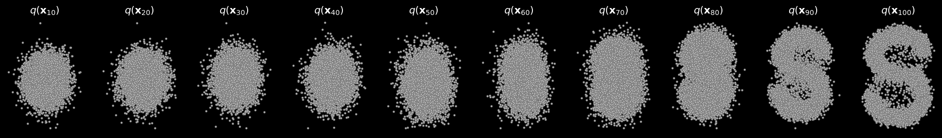
The codes in the next cells apply Gaussian noise to an image of the letter S over 100 steps. In the figure below, the images for every 10th step of the noise-adding process are shown.
[ ]:
from google.colab import drive
drive.mount('/content/drive')
Mounted at /content/drive
[ ]:
cd 'drive/MyDrive/Data_Science_Course/Fall_2023/Lecture_22-Diffusion_Models/helper_functions/'
/content/drive/MyDrive/Data_Science_Course/Fall_2023/Lecture_22-Diffusion_Models/helper_functions
[ ]:
# code from: https://github.com/azad-academy/denoising-diffusion-model

### Note: the code in the next cells for this example is not required for quizzes or assignments  ###

import numpy as np
from sklearn.datasets import make_s_curve
from helper_plot import hdr_plot_style
import torch
from utils import *

# create S curve
s_curve, _= make_s_curve(10**4, noise=0.1)
s_curve = s_curve[:, [0, 2]]/10.0

data = s_curve.T

# plot the S curve
hdr_plot_style()
plt.scatter(*data, alpha=0.5, color='white', edgecolor='gray', s=5)
plt.axis('off')

dataset = torch.Tensor(data.T).float()

[ ]:
num_steps = 100

# apply a sigmoid schedule for the beta parameter
betas = make_beta_schedule(schedule='sigmoid', n_timesteps=num_steps, start=1e-5, end=0.5e-2)

# substitute alphas
alphas = 1 - betas
alphas_prod = torch.cumprod(alphas, 0)
alphas_prod_p = torch.cat([torch.tensor([1]).float(), alphas_prod[:-1]], 0)
alphas_bar_sqrt = torch.sqrt(alphas_prod)
one_minus_alphas_bar_log = torch.log(1 - alphas_prod)
one_minus_alphas_bar_sqrt = torch.sqrt(1 - alphas_prod)
[ ]:
# draw a sample at step t, given an initial image x_0
def q_x(x_0, t, noise=None):
    if noise is None:
        noise = torch.randn_like(x_0)
    alphas_t = extract(alphas_bar_sqrt, t, x_0)
    alphas_1_m_t = extract(one_minus_alphas_bar_sqrt, t, x_0)
    return (alphas_t * x_0 + alphas_1_m_t * noise)
[ ]:
# plot the samples for steps 0, 10, 20, ..., 90
fig, axs = plt.subplots(1, 10, figsize=(24, 3))
for i in range(10):
    q_i = q_x(dataset, torch.tensor([i * 10]))
    axs[i].scatter(q_i[:, 0], q_i[:, 1], color='white', edgecolor='gray', s=5)
    axs[i].set_axis_off(); axs[i].set_title('$q(\mathbf{x}_{'+str(i*10)+'})$')

As mentioned above, we can obtain a sample at any desired step in the forward diffusion process, by applying the level of Gaussian noise directly to the initial image. The cell below shows the image at step 15.
[ ]:
# image in the 15th step
q_15 = q_x(dataset, torch.tensor([15]))
plt.scatter(q_15[:, 0], q_15[:, 1], color='white', edgecolor='gray', s=5);

22.3.2 Reverse Diffusion Process
The goal of the reverse diffusion process is to denoise the images from the forward diffusion process, i.e., start with a noisy image and obtain a clean image. Accurately calculating the reverse process \(q({x}_{t-1}|{x}_{t})\) is intractable, and therefore, text-to-image models apply deep neural networks to approximate the probability density function \(q({x}_{t-1}|{x}_{t})\) with a parameterized model \(p_{\theta}({x}_{t-1}|{x}_{t})\), where \(\theta\) denotes the parameters of the deep neural network model that are learned. The model takes as input a noisy image at step \({x}_{t}\) and predicts the mean \(\mu_\theta({x}_{t},t)\) and the variance \(\Sigma_\theta ({x}_{t},t)\) of a denoised image \({x}_{t-1}\).

Figure: Reverse diffusion process.
Example of Reverse Diffusion
The reverse diffusion process for the image S from the above example is presented below. The mathematical expressions for calculating the posteriors are omitted here, and can be found in reference [3]. The model is trained for 1,000 iterations, and the denoising images at steps 0, 250, 500, 750, and 1,000 are shown in the figure below. In the last row of images, we can see that the model begins with a noisy image on the left and it ends with a denoised image on the right.
[ ]:
posterior_mean_coef_1 = (betas * torch.sqrt(alphas_prod_p) / (1 - alphas_prod))
posterior_mean_coef_2 = ((1 - alphas_prod_p) * torch.sqrt(alphas) / (1 - alphas_prod))
posterior_variance = betas * (1 - alphas_prod_p) / (1 - alphas_prod)
posterior_log_variance_clipped = torch.log(torch.cat((posterior_variance[1].view(1, 1), posterior_variance[1:].view(-1, 1)), 0)).view(-1)

def q_posterior_mean_variance(x_0, x_t, t):
    coef_1 = extract(posterior_mean_coef_1, t, x_0)
    coef_2 = extract(posterior_mean_coef_2, t, x_0)
    mean = coef_1 * x_0 + coef_2 * x_t
    var = extract(posterior_log_variance_clipped, t, x_0)
    return mean, var
The U-Net model is imported in the next cell, and the model is trained for 1,000 iterations.
[ ]:
from model import ConditionalModel
from ema import EMA
import torch.optim as optim

model = ConditionalModel(num_steps)
optimizer = optim.Adam(model.parameters(), lr=1e-3)
# Create EMA model
ema = EMA(0.9)
ema.register(model)
# Batch size
batch_size = 128

# training
for t in range(1000):
    # X is a torch Variable
    permutation = torch.randperm(dataset.size()[0])
    for i in range(0, dataset.size()[0], batch_size):
        # Retrieve current batch
        indices = permutation[i:i+batch_size]
        batch_x = dataset[indices]
        # Compute the loss
        loss = noise_estimation_loss(model, batch_x,alphas_bar_sqrt,one_minus_alphas_bar_sqrt,num_steps)
        # Before the backward pass, zero all of the network gradients
        optimizer.zero_grad()
        # Backward pass: compute gradient of the loss with respect to parameters
        loss.backward()
        # Perform gradient clipping
        torch.nn.utils.clip_grad_norm_(model.parameters(), 1.)
        # Calling the step function to update the parameters
        optimizer.step()
        # Update the exponential moving average
        ema.update(model)
    # Print loss
    if (t % 250==0) or (t==999):
        print('Iteration:', t)
        x_seq = p_sample_loop(model, dataset.shape,num_steps,alphas,betas,one_minus_alphas_bar_sqrt)
        fig, axs = plt.subplots(1, 10, figsize=(24, 3))
        for i in range(1, 11):
            cur_x = x_seq[i * 10].detach()
            axs[i-1].scatter(cur_x[:, 0], cur_x[:, 1],color='white',edgecolor='gray', s=5);
            axs[i-1].set_axis_off();
            axs[i-1].set_title('$q(\mathbf{x}_{'+str(i*10)+'})$')
Iteration: 0
Iteration: 250
Iteration: 500
Iteration: 750
Iteration: 999


The gif image of the reverse diffusion process is shown below.

Figure: Animation of the reverse diffusion process.
U-Net Model for Reverse Diffusion
A U-Net model is used for the reverse diffusion phase. U-Net is a popular deep learning network for image segmentation. The name is due to the architecture that looks like the letter U. U-Net includes an encoder sub-network that extracts lower-dimensional representations, and a decoder sub-network that reconstructs the representations to full size images. I.e., the encoder first downsamples the input image (reducing its size), and afterward the decoder upsamples the representations to the size of the original image. Another important part of U-Net are the skip connections which connect the feature maps from the encoder to the decoder, and help with the gradient flow. When U-Net is used for image segmentation, the inputs are images, and the outputs are segmentation masks that segment the objects in the input images.

Figure: U-Net network.
In diffusion models, input to U-Net is a noisy image \({x}_{t}\) at a particular time step \(t\), and output by the model is the noise that has been added to the image in the previous time step of the forward diffusion process. By subtracting the predicted noise \(\epsilon_{t}\) from the input image \({x}_{t}\), the result is a denoised image \({x}_{t-1}\) at the previous time step. By repeating this process for every time step \(t\) from the final step \(T\) to the initial step \(0\), the model learns how to gradually create slightly less denoised images at each step. The final output for time step \(0\) is a fully denoised image \({x}_{0}\).
22.4 Text Encoder
To generate images based on a text prompt, text-to-image models employ text embeddings from a Language Model. In particular, the model CLIP (Contrastive Language Image Pretraining) has been used by several of these models.
CLIP employs a Transformer Network architecture. It is trained on a dataset of images and image captions, with an objective to match the text in image captions to the content in the corresponding images.

Figure: Images and captions dataset.
CLIP has an image encoder and a text encoder sub-network (shown in the figure). The two encoders convert the input pairs of images and image captions into image embeddings and text embeddings, respectively. During training, the model learns to group together image and text embeddings that belong to the same object. By repeating the training over a large dataset of images and image captions, the model updates the weights of the image and text encoders so that they output predictions that match the caption text and image content for the objects in the training dataset.

Figure: CLIP model.
22.5 Latent Diffusion Models
Latent Diffusion Models apply the diffusion process to a compressed image representation in a lower-dimensional space, instead of applying the diffusion process to the raw high-dimensional images. The lower-dimensional space is called latent space, hence the name for these models. Stable Diffusion is a Latent Diffusion Model.
The key advantage of Latent Diffusion Models is computational efficiency, due to processing small-size image representations. For instance, Stable Diffusion is trained on images of size 512x512 pixels, whereas the size of the image representations in the latent space is 64x64 pixels. Another advantage of performing the diffusion process in the latent space instead of the pixel space, is producing diverse images that preserve the semantic structure of the data.
An annotated figure of a Latent Diffusion Model is shown in the next figure. The components of the model are described next.

Figure: Latent diffusion model.
Perceptual Compression
The input image to the model \(x\) is shown in the upper left corner. The input image is in the pixel space, i.e., it consists of raw pixels. During the perceptual compression step, the image is projected into the latent space. For this step, an Encoder network \(\mathcal{E}\) is employed to produce a lower-dimensional representation of the input image \(z\) that has smaller dimensions.
Forward Diffusion Step
Forward diffusion process is applied to the latent representation of the image \(z\), by applying steps of gradually corrupting the image with Gaussian noise. The output of the forward diffusion step is a noise-corrupter image \(z_T\).
Semantic Compression
This step corresponds to the right-hand block in the figure, and typically employs a Language Model to capture the semantic structure in text and images. An example is the use of the image-caption CLIP model from the previous section. This model encodes the text prompt by the user into a compressed representation, denoted \(\tau_{\theta}\) in the figure. This compressed representation of the user’s prompt is used during the reverse diffusion step to control the visual content generated by the model and to guide the image generation process in order to ensure that the content in the denoised image corresponds to the text prompt.
Reverse Diffusion Step
The reverse diffusion step takes noisy images \(z_T\) and gradually removes the noise to generate clean images \(z\). As we mentioned, a U-Net model is typically employed for learning the denoising process. The reverse diffusion process is conditioned on the text representation \(\tau_{\theta}\) from the pretrained CLIP transformer model. I.e., conditioning the reverse diffusion means that the model guides the denoising process by mapping the compressed text representations to the intermediate layers of the U-Net via cross-attention layers. The cross-attention layers are similar to the self-attention mechanism in Transformer Networks, and they learn a set of Q (queries), K (keys), and V (values) matrices. The U-Net network also has added positional encodings into each block, which specify the diffusion timestep \(t\).
High-resolution Image Decoder
The obtained latent vector \(z\) is finally passed through a Decoder network \(\mathcal{D}\) to increase the resolution back to the size of the original image. I.e., the resulting image representation in the latent space is 64x64 pixels, and the decoder recovers it to a high-resolution image with 512x512 pixels size in the pixel space. The generated image is denoted \(\tilde{x}\) in the figure.
22.6 Generating Images with Stable Diffusion
The Stable Diffusion model trained by Stability.AI is available at Hugging Face. Let’s use this model to generate images. Note that in the above code in Section 22.2 we used an implementation of Stable Diffusion by Keras.
To use this model requires to login at Hugging Face and obtain a token. After that, you can simply download the diffusers and transformers packages, and provide text prompts to generate images.
[ ]:
!pip install -q huggingface-hub

from huggingface_hub import notebook_login
notebook_login()
[ ]:
!pip install -qq -U diffusers transformers accelerate
[ ]:
from diffusers import StableDiffusionPipeline
import torch

# set up the pipeline to generate images
pipe = StableDiffusionPipeline.from_pretrained("CompVis/stable-diffusion-v1-4", revision="fp16", torch_dtype=torch.float16).to('cuda')

prompt = "a photograph of an astronaut riding a horse"
# generate an image for the above prompt
pipe(prompt).images[0]
/usr/local/lib/python3.10/dist-packages/diffusers/pipelines/pipeline_utils.py:267: FutureWarning: You are loading the variant fp16 from CompVis/stable-diffusion-v1-4 via `revision='fp16'`. This behavior is deprecated and will be removed in diffusers v1. One should use `variant='fp16'` instead. However, it appears that CompVis/stable-diffusion-v1-4 currently does not have the required variant filenames in the 'main' branch.
 The Diffusers team and community would be very grateful if you could open an issue: https://github.com/huggingface/diffusers/issues/new with the title 'CompVis/stable-diffusion-v1-4 is missing fp16 files' so that the correct variant file can be added.
  warnings.warn(
vae/diffusion_pytorch_model.safetensors not found
/usr/local/lib/python3.10/dist-packages/transformers/models/clip/feature_extraction_clip.py:28: FutureWarning: The class CLIPFeatureExtractor is deprecated and will be removed in version 5 of Transformers. Please use CLIPImageProcessor instead.
  warnings.warn(
`text_config_dict` is provided which will be used to initialize `CLIPTextConfig`. The value `text_config["id2label"]` will be overriden.
`text_config_dict` is provided which will be used to initialize `CLIPTextConfig`. The value `text_config["bos_token_id"]` will be overriden.
`text_config_dict` is provided which will be used to initialize `CLIPTextConfig`. The value `text_config["eos_token_id"]` will be overriden.

[ ]:
prompt = "a cute magical flying dog, fantasy art, golden color, high quality, highly detailed, elegant, sharp focus," \
    "concept art, character concepts, digital painting, mystery, adventure"
# generate an image for the above prompt
pipe(prompt).images[0]

The results from text-to-image models can vary based on the text prompt. Prompt engineering involves customizing the text prompts to influence the generated images. Examples of prompt engineering include specifying the painting style of the image type, lighting, focus, etc.
Appendix
The material in the Appendix is not required for quizzes and assignments.
Interpolation Between Prompts
Text-to-image models can be used to interpolate between the embedding representations of different text prompts. This is referred to as latent space walking or latent space exploration because the model samples data points in the latent space and incrementally changes the latent representation to reach from one text prompt to another text prompt.
One application is shown below, where each sampled point is saved as a frame, and a gif animation is created that shows the latent space walking between two prompts.
[ ]:
# Code from: https://github.com/svpino/stable-diffusion/blob/main/stable-diffusion.ipynb

PROMPT1 = "a ford truck"
PROMPT2 = "an electric car"

# number of interpolation steps between the two text prompts
INTERPOLATION_STEPS = 42

# number of frames per second
FRAMES_PER_SECOND = 10

# number of diffusion steps
DIFFUSION_STEPS = 25

# name of the file
ANIMATION_FILENAME = "animation.gif"

SEED = 42
[ ]:
import tensorflow as tf
from PIL import Image

# random noise patch
noise = tf.random.normal((512 // 8, 512 // 8, 4), seed=SEED)

# encoded vectors for the two text prompts
encoding1 = tf.squeeze(model.encode_text(PROMPT1))
encoding2 = tf.squeeze(model.encode_text(PROMPT2))

# generate the interpolation steps between the two encoded prompts
interpolated_encodings = tf.linspace(encoding1, encoding2, INTERPOLATION_STEPS)

# split the encodings into batches
batch_size = 3
batches = INTERPOLATION_STEPS // batch_size
encodings = tf.split(interpolated_encodings, batches)

animation = []
for batch in range(batches):
    # generate images
    images = model.generate_image(
        encodings[batch],
        batch_size=batch_size,
        num_steps=DIFFUSION_STEPS,
        diffusion_noise=noise,
    )

    # add the images to the animation
    animation.extend(map(lambda image: Image.fromarray(image), images))

def export_as_gif(images, filename, frames_per_second=10):
    """
    Exports the supplied images as a GIF animation.
    """
    images += images[2:-1][::-1]
    images[0].save(filename, save_all=True, append_images=images[1:],
        duration=1000 // frames_per_second, loop=0)

# Export the animation as a GIF and display it on the screen.
export_as_gif(animation, ANIMATION_FILENAME, frames_per_second=FRAMES_PER_SECOND)
25/25 [==============================] - 42s 2s/step
25/25 [==============================] - 43s 2s/step
25/25 [==============================] - 43s 2s/step
25/25 [==============================] - 43s 2s/step
25/25 [==============================] - 43s 2s/step
25/25 [==============================] - 44s 2s/step
25/25 [==============================] - 44s 2s/step
25/25 [==============================] - 44s 2s/step
25/25 [==============================] - 44s 2s/step
25/25 [==============================] - 44s 2s/step
25/25 [==============================] - 44s 2s/step
25/25 [==============================] - 44s 2s/step
25/25 [==============================] - 44s 2s/step
25/25 [==============================] - 44s 2s/step

Figure: Latent space walking from a Ford truck to an electric car.
References
High-performance image generation using Stable Diffusion in KerasCV, available at https://keras.io/guides/keras_cv/generate_images_with_stable_diffusion/.
Diffusion Models Made Easy, J. Rafid Siddiqui, available at https://towardsdatascience.com/diffusion-models-made-easy-8414298ce4da.
How Diffusion Models Work: The Math From Scratch, available at https://theaisummer.com/diffusion-models/.
The Illustrated Stable Diffusion, Jay Alammar, available at https://jalammar.github.io/illustrated-stable-diffusion/.
What are Stable Diffusion Models and Why are they a Step Forward for Image Generation?, J. Rafid Siddiqui, available at https://towardsdatascience.com/what-are-stable-diffusion-models-and-why-are-they-a-step-forward-for-image-generation-aa1182801d46.
Generating Images using Stable Diffusion, available at https://github.com/svpino/stable-diffusion/blob/main/stable-diffusion.ipynb.
BACK TO TOP