Lecture 17 - Model Selection, Hyperparameter Tuning

• 17.1 Model Selection

• 17.2 Evaluate the Impact of the Learning Rate

  • 17.2.1 Learning Rate Finder

• 17.3 Callbacks

  • 17.3.1 Early Stopping

  • 17.3.2 Save Checkpoint

  • 17.3.3 Reduce Learning Rate on Plateau

  • 17.3.4 Learning Rate Scheduler

• 17.4 Grid Search

• 17.5 Keras Tuner

• 17.6 AutoML

• References

17.1 Model Selection

Model selection in Machine Learning is selecting one final model for a given task, e.g., that will be deployed in production. In general, selecting the “best” model should be based not only on the obtained values of relevant performance metrics (accuracy, specificity, sensitivity), but also based on other considerations, such as computational expense, available resources, model complexity, maintainability, and similar.

An important phase in selecting a candidate Machine Learning model is hyperparameter tuning. In the previous lecture on scikit-learn, we mentioned that parameters (weights) of the model have values that are updated in an iterative process during training, whereas hyperparameters (tuning parameters) are a set of parameters that control the complexity and performance of the model, and are selected (tuned) by the user. The hyperparameters are not updated during model training, and they stay constant. Hyperparameter tuning (also known as hypertuning) is the process of selecting hyperparameter values to find a model that generalizes well to unseen data. In the previous lectures, we explained that scikit-learn offers functions for Grid Search and Random Search, which search for solutions over different values of the hyperparameters and select an optimal set of hyperparameters for a given performance metric.

Another important aspect for model selection is the evaluation of model performance. It is particularly important to evaluate candidate models on unseen data during training, and this is typically achieved by splitting the available data into training and test datasets. We also learned that k-fold cross-validation can be used to draw folds from the available data, and evaluate the models on multiple different folds by resampling the available data. With k-fold cross-validation, each data point can appear only in one of the folds when evaluating the model performance.

Model selection in general can involve various data preprocessing techniques, evaluating different feature engineering strategies, applying Ensemble Methods to aggregate the predictions from several individual Machine Learning models, etc.

In this lecture, we will focus on hyperparameter tuning with neural networks. Namely, neural networks are more sensitive to hyperparameter tuning than conventional Machine Learning models (such as Liner Regression, k-Nearest Neighbors, etc.). We saw in the previous lectures that even if we use default values for the models in scikit-learn without any hyperparameter tuning, the models can still achieve solid performance. This is rarely the case with neural networks, as they usually require at least some hyperparameter tuning.

One note is to not confuse hyperparameter tuning with model fine-tuning, which refers to using a pretrained model on a large dataset and fine-tuning the model parameters on a smaller dataset.

Hyperparameters in Neural Networks

Let’s examine again the ConvNet that we used in a previous lecture to classify images in the CIFAR-10 dataset, and let’s try to identify the hyperparameters of the model.

# define the layers in the model
inputs = Input(shape=(32, 32, 3))
conv1a = Conv2D(filters=32, kernel_size=3, padding='same')(inputs)
conv1b = Conv2D(filters=32, kernel_size=3, padding='same')(conv1a)
pool1 = MaxPooling2D()(conv1b)
conv2a = Conv2D(filters=64, kernel_size=3, padding='same')(pool1)
conv2b = Conv2D(filters=64, kernel_size=3, padding='same')(conv2a)
pool2 = MaxPooling2D()(conv2b)
conv3a = Conv2D(filters=128, kernel_size=3, padding='same')(pool2)
conv3b = Conv2D(filters=128, kernel_size=3, padding='same')(conv3a)
pool3 = MaxPooling2D()(conv3b)
flat = Flatten()(pool3)
dense1 = Dense(128, activation='relu')(flat)
dropout1 = Dropout(0.25)(dense1)
dense2 = Dense(64, activation='relu')(dropout1)
dropout2  = Dropout(0.25)(dense2)
outputs = Dense(10, activation='softmax')(dropout2)

# define the model with inputs and outputs
cifar_cnn = Model(inputs, outputs)

# compile the model
cifar_cnn.compile(optimizer=Adam(learning_rate=1e-3), loss='categorical_crossentropy',  metrics=['accuracy'])

# train the model
cifar_cnn.fit(train_data, train_label_onehot, epochs=10, batch_size=128)

Hyperparameters in the above model include:

• Learning rate of the optimizer

• Batch size

• Number of training epochs

• Number of Convolutional layers

• Number of convolutional filters in the Convolutional layers

• Kernel size of the convolutional filters

• Type of padding in the Convolutional layers

• Number of Dense layers

• Number of neurons in each Dense layer

• Type of activation functions used in the layers

• Number of Dropout layers

• Dropout rate in the Dropout layers

• Type of optimizer (e.g., Adam, SGD, Nadam, RMSProp)

• Other parameters used in the optimizer (e.g., momentum)

• Type of initialization for the parameters in the model

There can be other hyperparameters depending on the network, however, one immediate observation is that neural networks have a large number of hyperparameters, and tuning all hyperparameters can be challenging as it may take significant time and resources.

On the other hand, not all of the hyperparameters have significant impact on the performance of the model. Out of all hyperparameters, probably the most important is the learning rate, and in most cases, some tuning of the learning rate is required. In this lecture we will present techniques for hyperparameter tuning of a ConvNet model built with Keras and TensorFlow.

17.2 Evaluate the Impact of the Learning Rate

Loading a Custom Image Dataset in Keras

In previous lectures we worked with datasets that are built-in in Keras or scikit-learn and that can be directly loaded. Let’s look at loading a custom dataset that is not part of the popular ML libraries. The dataset is saved in a folder on my Google Drive, therefore I need to first mount the Google Drive in order to access the folder with the images.

For this lecture, we will use the LFW dataset (Labeled Faces in the Wild), which consists of about 5,000 images of 62 celebrities. The next cells load the dataset and plot a few images to make sure that the labels are correct.

# mount the google drive
from google.colab import drive
drive.mount('/content/drive')

Drive already mounted at /content/drive; to attempt to forcibly remount, call drive.mount("/content/drive", force_remount=True).

# import packages
import numpy as np
import matplotlib.pyplot as plt
import tensorflow as tf
from tensorflow import keras
from keras.utils import load_img, img_to_array
import os
from os import listdir
import csv
import natsort

# Print the version of tf
print("TensorFlow version:{}".format(tf.__version__))

TensorFlow version:2.14.0

# Path to the directory containing the dataset
!unzip -uq 'drive/MyDrive/Data_Science_Course/Fall_2023/Lecture_17-Model_Selection,Tuning/data/LFW-dataset.zip' -d 'sample_data/'

# Directories
train_dir = 'sample_data/LFW-dataset/Train/'
test_dir = 'sample_data/LFW-dataset/Test/'
val_dir = 'sample_data/LFW-dataset/Validation/'
labels_dir = 'sample_data/LFW-dataset/'

# Size of images (pixel width and height)
image_size = 100

# Function for loading the images
def load_imgs(path):
    # List of all images in the folder
    imgList = listdir(path)
    # Make sure that the images are sorted in ascending order
    imgList=natsort.natsorted(imgList)
    # Number of images
    number_imgs = len(imgList)
    # Initialize numpy arrays for the images
    images = np.zeros((number_imgs, image_size, image_size, 3))
    # Read the images
    for i in range(number_imgs):
        tmp_img = load_img(path + imgList[i], target_size=(image_size, image_size, 3))
        img = img_to_array(tmp_img)
        images[i] = img/255.0
    return images

# Call the above function to load the images as numpy arrays
imgs_train = load_imgs(train_dir)
imgs_test = load_imgs(test_dir)
imgs_val = load_imgs(val_dir)

# Load the labels as numpy arrays
labels_train = np.genfromtxt(labels_dir + "train_labels.csv", delimiter=',', dtype=np.int32)
labels_test = np.genfromtxt(labels_dir + "test_labels.csv", delimiter=',', dtype=np.int32)
labels_val = np.genfromtxt(labels_dir + "val_labels.csv", delimiter=',', dtype=np.int32)

# Display the shapes of train, validation, and test datasets
print('Images train shape: {} - Labels train shape: {}'.format(imgs_train.shape, labels_train.shape))
print('Images validation shape: {} - Labels validation shape: {}'.format(imgs_val.shape, labels_val.shape))
print('Images test shape: {} - Labels test shape: {}'.format(imgs_test.shape, labels_test.shape))

# Display the range of images (to make sure they are in the [0, 1] range)
print('\nMax pixel value', np.max(imgs_train))
print('Min pixel value', np.min(imgs_train))
print('Average pixel value', np.mean(imgs_train))
print('Data type', imgs_train[0].dtype)

Images train shape: (3043, 100, 100, 3) - Labels train shape: (3043,)
Images validation shape: (1021, 100, 100, 3) - Labels validation shape: (1021,)
Images test shape: (1049, 100, 100, 3) - Labels test shape: (1049,)

Max pixel value 1.0
Min pixel value 0.0
Average pixel value 0.47390351913451484
Data type float64

# Read the names of the celebrities in the dataset (there are 62 celebrities)
name_list = []
with open(labels_dir+'name_list.csv', 'r') as f:
    reader = csv.reader(f)
    for row in reader:
        name_list.append(row[1])

# Plot a few images to check if the the labels are correct
# There are a few bad images in the dataset, it needs to be cleaned
plt.figure(figsize=(9, 6))
for n in range(9):
    i = np.random.randint(0, len(imgs_train), 1)
    ax = plt.subplot(3, 3, n+1)
    plt.imshow(imgs_train[i[0]])
    plt.title('Label:' + str(name_list[labels_train[i[0]]]))
    plt.axis('off')

Define the Model

We will use a pretrained VGG-16 model, and we will just add a classifier with 3 Dense layers on top of the model to fine-tune it to the LFW dataset.

from keras.models import Model
from keras.layers import Dense, GlobalAveragePooling2D, Dropout
from keras.optimizers import Adam
from keras.callbacks import EarlyStopping, ModelCheckpoint, ReduceLROnPlateau, LearningRateScheduler
from keras.applications import vgg16

import datetime
now = datetime.datetime.now

def Network():

    base_model = vgg16.VGG16(weights='imagenet', include_top=False, input_shape=(image_size, image_size, 3))

    # Add a global spatial average pooling layer
    x = base_model.output
    x = GlobalAveragePooling2D()(x)
    # Add fully-connected layers
    x = Dense(1024, activation='relu')(x)
    x = Dropout(0.25)(x)
    x = Dense(256, activation='relu')(x)
    x = Dropout(0.25)(x)
    # Add a softmax layer
    predictions = Dense(62, activation='softmax')(x)

    # The model
    model = Model(inputs=base_model.input, outputs=predictions)

    return model

Let’s define a function for plotting the accuracy and loss called plot_accuracy_loss, which we can call with different models to examine the learning curves.

def plot_accuracy_loss():
    # plot the accuracy and loss
    train_loss = history.history['loss']
    val_loss = history.history['val_loss']
    acc = history.history['accuracy']
    val_acc = history.history['val_accuracy']

    epochsn = np.arange(1, len(train_loss)+1,1)
    plt.figure(figsize=(12, 4))

    plt.subplot(1,2,1)
    plt.plot(epochsn, acc, 'b', label='Training Accuracy')
    plt.plot(epochsn, val_acc, 'r', label='Validation Accuracy')
    plt.grid(color='gray', linestyle='--')
    plt.legend()
    plt.title('ACCURACY')
    plt.xlabel('Epochs')
    plt.ylabel('Accuracy')

    plt.subplot(1,2,2)
    plt.plot(epochsn,train_loss, 'b', label='Training Loss')
    plt.plot(epochsn,val_loss, 'r', label='Validation Loss')
    plt.grid(color='gray', linestyle='--')
    plt.legend()
    plt.title('LOSS')
    plt.xlabel('Epochs')
    plt.ylabel('Loss')
    plt.show()

Learning rate = 1e-4, Epochs = 10

In Lecture 15, we explained that most NNs employ a version of the Gradient Descent algorithm for updating the network parameters during training, depicted in the figure below. The learning rate determines the size of the updates at each step, i.e., it controls how fast the network parameters are updated.

Figure: Gradient descent algorithm.

If the learning rate is too small, the algorithm will take many epochs to converge, and it may even get stuck into a local minima. If the learning rate is too high, the algorithm may jump over the best solutions and may not be able to converge to good solutions.

Figure: Impact of the learning rate. Source: https://www.bdhammel.com/learning-rates/

In the previous lectures, we used the following code to compile the models, which uses the Adam optimizer, but we didn’t specify the learning rate of the optimizer. For the implementation of Adam in Keras, the default learning rate is 1e-3.

model.compile(optimizer='adam',
              loss='sparse_categorical_crossentropy',
              metrics=['accuracy'])

If we would like to use another value for the learning rate, then we will need to import the Adam optimizer, and compile the model with:

from keras.optimizers import Adam
model.compile(optimizer = Adam(learning_rate=VALUE),
              loss='sparse_categorical_crossentropy',
              metrics=['accuracy'])

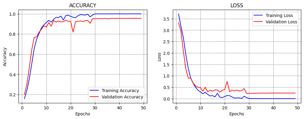
The following code trains a model for 10 epochs with a learning rate of 1e-4 = 0.0001. We have selected this learning rate because we know that it works well for this combination of model and data.

We can see that the model achieved close to 90% accuracy on the test set, and the training took about 1 minute. From the plots of the accuracy and loss curves, we can tell that 10 epochs are not sufficient for training the model, because at the end of the 10th epoch, the accuracy was still increasing and the loss was decreasing.

LEARNING_RATE = 1e-4
EPOCHS_NUM = 10

# create a model
model = Network()

# compile the model
model.compile(optimizer = Adam(learning_rate=LEARNING_RATE), loss='sparse_categorical_crossentropy', metrics=['accuracy'])

# fit model
t = now()
history = model.fit(imgs_train, labels_train, batch_size=32, epochs=EPOCHS_NUM,
                     validation_data=(imgs_val, labels_val), verbose=0)
print('\nTraining time: %s' % (now() - t))

# evaluate on test data
evals_test = model.evaluate(imgs_test, labels_test)
print("Classification Accuracy: ", 100*evals_test[1])

# plot the accuracy and loss
plot_accuracy_loss()

Training time: 0:00:44.932419
33/33 [==============================] - 1s 21ms/step - loss: 0.3862 - accuracy: 0.8990
Classification Accuracy:  89.89514112472534

Learning rate = 1e-4, Epochs = 30

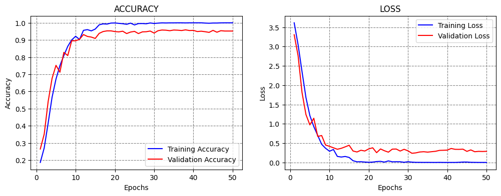
Let’s train the model for 30 epochs using the same learning rate to see if this number of epochs would be sufficient.

From the results we can see that the model achieved 94% accuracy, and the training took about 2 minutes.

Based on the learning curves, at epoch 30 the validation accuracy and loss were converging to a plateau level, and it was unclear if training the model for more than 30 epochs would improve the performance. An alternative is to use Early Stopping callback, so that the training is stopped automatically (e.g., when the validation loss stops decreasing). Such case is shown in a subsequent section.

LEARNING_RATE = 1e-4
EPOCHS_NUM = 30

model = Network()
model.compile(optimizer = Adam(learning_rate=LEARNING_RATE), loss='sparse_categorical_crossentropy', metrics=['accuracy'])

# fit model
t = now()
history = model.fit(imgs_train, labels_train, batch_size=32, epochs=EPOCHS_NUM,
                     validation_data=(imgs_val, labels_val), verbose=0)
print('\nTraining time: %s' % (now() - t))

# Evaluate on test data
evals_test = model.evaluate(imgs_test, labels_test)
print("Classification Accuracy: ", 100*evals_test[1])

# plot the accuracy and loss
plot_accuracy_loss()

Training time: 0:01:49.333017
33/33 [==============================] - 0s 12ms/step - loss: 0.3438 - accuracy: 0.9428
Classification Accuracy:  94.28026676177979

Learning rate = 1e-3, Epochs = 20

Next, let’s try to train the model using different learning rates, for instance, by increasing the learning rate to 1e-3 = 0.001.

Increasing the learning rate will cause the model to apply larger values for the update of the parameters during the training. We can expect that the training will converge faster, and we can use a smaller number of epochs.

However, large learning rates can cause the model to update the parameters too fast, as in this case. As we can see, the model achieved only 16.87% accuracy, and the accuracy curves did not improve after that level.

LEARNING_RATE = 1e-3
EPOCHS_NUM = 20

model = Network()
model.compile(optimizer = Adam(learning_rate=LEARNING_RATE), loss='sparse_categorical_crossentropy', metrics=['accuracy'])

# fit model
t = now()
history = model.fit(imgs_train, labels_train, batch_size=32, epochs=EPOCHS_NUM,
                     validation_data=(imgs_val, labels_val), verbose=0)
print('\nTraining time: %s' % (now() - t))

# Evaluate on test data
evals_test = model.evaluate(imgs_test, labels_test)
print("Classification Accuracy: ", 100*evals_test[1])

# plot the accuracy and loss
plot_accuracy_loss()

Training time: 0:01:13.950914
33/33 [==============================] - 0s 11ms/step - loss: 3.7229 - accuracy: 0.1687
Classification Accuracy:  16.873212158679962

Learning rate = 1e-2, Epochs = 10

If we increase the learning rate even further to 0.01, we can expect that training will fail, since we saw that even a learning rate of 0.001 was too high. Based on the learning curves, we can tell that the learning is too fast and too aggressive.

LEARNING_RATE = 1e-2
EPOCHS_NUM = 10

model = Network()
model.compile(optimizer = Adam(learning_rate=LEARNING_RATE), loss='sparse_categorical_crossentropy', metrics=['accuracy'])

# fit model
t = now()
history = model.fit(imgs_train, labels_train, batch_size=32, epochs=EPOCHS_NUM,
                     validation_data=(imgs_val, labels_val), verbose=0)
print('\nTraining time: %s' % (now() - t))

# Evaluate on test data
evals_test = model.evaluate(imgs_test, labels_test)
print("Classification Accuracy: ", 100*evals_test[1])

# plot the accuracy and loss
plot_accuracy_loss()

Training time: 0:00:39.685677
33/33 [==============================] - 0s 12ms/step - loss: 3.7224 - accuracy: 0.1687
Classification Accuracy:  16.873212158679962

Learning rate = 1e-5, Epochs = 50

Let’s try the opposite case, and reduce the learning rate to 1e-5 = 0.00001. Smaller learning rates produce smaller updates of the model parameters, and slower learning. This may avoid the problems of learning too fast when large learning rates are used.

This model achieved similar accuracy as with the 1e-4 learning rate. Also, the learning curves look good, because the accuracy and loss gradually change, and the validation curves follow the training curves.

LEARNING_RATE = 1e-5
EPOCHS_NUM = 50

model = Network()
model.compile(optimizer = Adam(learning_rate=LEARNING_RATE), loss='sparse_categorical_crossentropy', metrics=['accuracy'])

# fit model
t = now()
history = model.fit(imgs_train, labels_train, batch_size=32, epochs=EPOCHS_NUM,
                     validation_data=(imgs_val, labels_val), verbose=0)
print('\nTraining time: %s' % (now() - t))

# Evaluate on test data
evals_test = model.evaluate(imgs_test, labels_test)
print("Classification Accuracy: ", 100*evals_test[1])

# plot the accuracy and loss
plot_accuracy_loss()

Training time: 0:02:58.985777
33/33 [==============================] - 0s 12ms/step - loss: 0.2841 - accuracy: 0.9409
Classification Accuracy:  94.08960938453674

Learning rate = 1e-6, Epochs = 50

Next, let’s reduce the learning rate even further to 1e-6.

Although smaller learning rates avoid training failure when we use overly large learning rates, using very small learning rates does not necessarily lead to improved performance, since the learning can be too slow.

Based on the learning curves, we can tell that at the end of epoch 50 the model parameters were gradually being updated, and that with this learning rate we would need to train the model for at least 200 or 300 epochs to reach convergence, or maybe even more.

LEARNING_RATE = 1e-6
EPOCHS_NUM = 50

model = Network()
model.compile(optimizer = Adam(learning_rate=LEARNING_RATE), loss='sparse_categorical_crossentropy', metrics=['accuracy'])

# fit model
t = now()
history = model.fit(imgs_train, labels_train, batch_size=32, epochs=EPOCHS_NUM,
                     validation_data=(imgs_val, labels_val), verbose=0)
print('\nTraining time: %s' % (now() - t))

# Evaluate on test data
evals_test = model.evaluate(imgs_test, labels_test)
print("Classification Accuracy: ", 100*evals_test[1])

# plot the accuracy and loss
plot_accuracy_loss()

Training time: 0:02:58.017459
33/33 [==============================] - 0s 12ms/step - loss: 1.3921 - accuracy: 0.6969
Classification Accuracy:  69.68541741371155

17.2.1 Learning Rate Finder

There are several tools for estimating the learning rate, such as LRFinder in Keras. This function changes the learning rate in a range of values, typically starting with a very small learning rate and increasing it to a high learning rate. The model is trained and evaluated only for a few epochs using different learning rates. Based on a plot of the loss for different learning rates, this function can help to find a suitable learning rate, that can afterward be used to fully train the model.

For the task at hand, the plot of loss versus learning rate is shown below. The best learning rate is the one when the loss is reducing the fastest, and has the largest slope. From the graph, this value is about \(10^{-4}\).

Although such tools can identify a range of suitable values for the learning rate, they should be used with caution, and the users should still run candidate models in the suggested range to fully evaluate the model performance.

!git clone https://github.com/WittmannF/LRFinder.git

Cloning into 'LRFinder'...
remote: Enumerating objects: 71, done.
remote: Total 71 (delta 0), reused 0 (delta 0), pack-reused 71
Receiving objects: 100% (71/71), 447.02 KiB | 12.08 MiB/s, done.
Resolving deltas: 100% (24/24), done.

from LRFinder.keras_callback import LRFinder

model = Network()
model.compile(optimizer='Adam', loss='sparse_categorical_crossentropy', metrics=['accuracy'])

# Perform the Learning Rate Range Test
lr_finder = LRFinder(min_lr=1e-6, max_lr=1e-2)

model.fit(imgs_train, labels_train, batch_size=32, callbacks=[lr_finder], epochs=2)

Epoch 1/2
 6/96 [>.............................] - ETA: 11s - loss: 4.1732 - accuracy: 0.0000e+00

WARNING:tensorflow:Callback method `on_train_batch_end` is slow compared to the batch time (batch time: 0.0407s vs `on_train_batch_end` time: 0.0935s). Check your callbacks.

96/96 [==============================] - 36s 122ms/step - loss: 4.1457 - accuracy: 0.0214
Epoch 2/2
96/96 [==============================] - 12s 120ms/step - loss: 3660.4465 - accuracy: 0.0796

<keras.callbacks.History at 0x7f5c50298650>

17.3 Callbacks

Callbacks in programming languages are functions that allow for conditional processing within another function. I.e., they allow to perform some operations during the execution of another function, based on some conditions.

In ML, callbacks are used to monitor the model performance at various stages of training and take certain actions (e.g., at the start or end of an epoch, before or after processing a single batch, etc.). Such actions can include saving the model to the disk after a certain number of epochs, obtaining a view of the internal states of the model and relevant statistics during training, writing logs after every batch of training data to monitor performance metrics, etc. Most ML libraries provide a callback class which allows users to create custom callbacks.

So far we worked with the history callback in Keras, which stores the values of the loss and the metric at each epoch, and its atribute history.history allows to plot the learning curves of a model. Also, in the lecture on ConvNets we explained how the EarlyStopping callback works. The next section provides additional examples of applying callbacks in Keras.

17.3.1 Early Stopping

As we know, using Early Stopping callback is often beneficial, since we don’t need to guess the optimal number of epochs to train the model. Instead, the callback will terminate the training when a selected metric is not improving. In the next cell, we specified to stop the training when the validation loss does not improve for 20 epochs (patience argument). We set the EPOCH_NUM argument to 1000, although we know that the model will terminate after about 50-60 epochs. Therefore, the number of epochs is not very important when we use this callback, it only needs to be large enough so that the training is not stopped prematurely.

This model achieved 91.13% accuracy. However, from the accuracy curve it seems that the accuracy was higher in the previous epoch, and it just dropped in the last epoch. We will see next how to avoid this by using CheckPoint callback.

LEARNING_RATE = 1e-4
EPOCHS_NUM = 1000

model = Network()
model.compile(optimizer=Adam(learning_rate=LEARNING_RATE), loss='sparse_categorical_crossentropy', metrics=['accuracy'])

# fit model
t = now()
callbacks = [EarlyStopping(monitor='val_loss', patience=20)]
history = model.fit(imgs_train, labels_train, batch_size=32, epochs=EPOCHS_NUM,
                     validation_data=(imgs_val, labels_val), verbose=0, callbacks=callbacks)
print('\nTraining time: %s' % (now() - t))

# Evaluate on test data
evals_test = model.evaluate(imgs_test, labels_test)
print("Classification Accuracy: ", 100*evals_test[1])

# plot the accuracy and loss
plot_accuracy_loss()

Training time: 0:04:01.178825
33/33 [==============================] - 0s 12ms/step - loss: 0.4387 - accuracy: 0.9256
Classification Accuracy:  92.56434440612793

17.3.2 Save CheckPoint

CheckPoint callback saves a checkpoint of the model (i.e., the model parameters) after every epoch when a monitored metric does not improve. We set the metrics to be the validation loss, and the values of the model parameters will be saved at the specified filepath. This can be useful if training the model takes hours, where if something goes wrong, we can just resume the training from a checkpoint.

We choose to set verbose=1 for the callback, to output the epochs at which a checkpoint is saved.

At the beginning of the training, the checkpoint will be saved after every epoch, and after the model reaches a plateau, a new checkpoint will be saved only when there is an improvement in the performance, by overwriting the latest checkpoint.

LEARNING_RATE = 1e-4
EPOCHS_NUM = 50

model = Network()
model.compile(optimizer=Adam(learning_rate=LEARNING_RATE), loss='sparse_categorical_crossentropy', metrics=['accuracy'])

# fit model
t = now()
callbacks = ModelCheckpoint(filepath='sample_data/model_celeb.h5', monitor='val_loss', mode='min',
                            save_weights_only=True, save_best_only=True, verbose=1)
history = model.fit(imgs_train, labels_train, batch_size=32, epochs=EPOCHS_NUM,
                     validation_data=(imgs_val, labels_val), verbose=0, callbacks=[callbacks])
print('Training time: %s' % (now() - t))

# Evaluate on test data
evals_test = model.evaluate(imgs_test, labels_test)
print("Classification Accuracy: ", 100*evals_test[1])

# plot the accuracy and loss
plot_accuracy_loss()

Epoch 1: val_loss improved from inf to 3.32760, saving model to sample_data/model_celeb.h5

Epoch 2: val_loss improved from 3.32760 to 3.08174, saving model to sample_data/model_celeb.h5

Epoch 3: val_loss improved from 3.08174 to 2.40263, saving model to sample_data/model_celeb.h5

Epoch 4: val_loss improved from 2.40263 to 1.87908, saving model to sample_data/model_celeb.h5

Epoch 5: val_loss improved from 1.87908 to 1.77787, saving model to sample_data/model_celeb.h5

Epoch 6: val_loss improved from 1.77787 to 1.03076, saving model to sample_data/model_celeb.h5

Epoch 7: val_loss improved from 1.03076 to 0.86254, saving model to sample_data/model_celeb.h5

Epoch 8: val_loss improved from 0.86254 to 0.83952, saving model to sample_data/model_celeb.h5

Epoch 9: val_loss improved from 0.83952 to 0.76099, saving model to sample_data/model_celeb.h5

Epoch 10: val_loss improved from 0.76099 to 0.45982, saving model to sample_data/model_celeb.h5

Epoch 11: val_loss improved from 0.45982 to 0.39744, saving model to sample_data/model_celeb.h5

Epoch 12: val_loss improved from 0.39744 to 0.36517, saving model to sample_data/model_celeb.h5

Epoch 13: val_loss improved from 0.36517 to 0.35960, saving model to sample_data/model_celeb.h5

Epoch 14: val_loss did not improve from 0.35960

Epoch 15: val_loss did not improve from 0.35960

Epoch 16: val_loss did not improve from 0.35960

Epoch 17: val_loss improved from 0.35960 to 0.33312, saving model to sample_data/model_celeb.h5

Epoch 18: val_loss did not improve from 0.33312

Epoch 19: val_loss did not improve from 0.33312

Epoch 20: val_loss improved from 0.33312 to 0.31346, saving model to sample_data/model_celeb.h5

Epoch 21: val_loss did not improve from 0.31346

Epoch 22: val_loss did not improve from 0.31346

Epoch 23: val_loss did not improve from 0.31346

Epoch 24: val_loss improved from 0.31346 to 0.30755, saving model to sample_data/model_celeb.h5

Epoch 25: val_loss did not improve from 0.30755

Epoch 26: val_loss did not improve from 0.30755

Epoch 27: val_loss did not improve from 0.30755

Epoch 28: val_loss did not improve from 0.30755

Epoch 29: val_loss did not improve from 0.30755

Epoch 30: val_loss did not improve from 0.30755

Epoch 31: val_loss improved from 0.30755 to 0.28651, saving model to sample_data/model_celeb.h5

Epoch 32: val_loss did not improve from 0.28651

Epoch 33: val_loss did not improve from 0.28651

Epoch 34: val_loss did not improve from 0.28651

Epoch 35: val_loss did not improve from 0.28651

Epoch 36: val_loss did not improve from 0.28651

Epoch 37: val_loss improved from 0.28651 to 0.26158, saving model to sample_data/model_celeb.h5

Epoch 38: val_loss did not improve from 0.26158

Epoch 39: val_loss did not improve from 0.26158

Epoch 40: val_loss did not improve from 0.26158

Epoch 41: val_loss improved from 0.26158 to 0.25302, saving model to sample_data/model_celeb.h5

Epoch 42: val_loss did not improve from 0.25302

Epoch 43: val_loss did not improve from 0.25302

Epoch 44: val_loss did not improve from 0.25302

Epoch 45: val_loss did not improve from 0.25302

Epoch 46: val_loss did not improve from 0.25302

Epoch 47: val_loss did not improve from 0.25302

Epoch 48: val_loss improved from 0.25302 to 0.23428, saving model to sample_data/model_celeb.h5

Epoch 49: val_loss improved from 0.23428 to 0.22223, saving model to sample_data/model_celeb.h5

Epoch 50: val_loss did not improve from 0.22223
Training time: 0:03:01.450305
33/33 [==============================] - 0s 11ms/step - loss: 0.2903 - accuracy: 0.9561
Classification Accuracy:  95.61486840248108

17.3.3 Reduce Learning Rate On Plateau

ReduceLROnPlateau stands for Reduce Learning Rate on Plateau. It is another very useful callback, since prior works have reported that training models generally benefits from using larger learning rate at the beginning of the training, and gradually reducing the learning rate when the training does not improve.

This is exactly what this callback does. In the next call, the learning rate is initially set to 1e-4=0.0001. ReduceLROnPlateau has a patience of 10 epochs, factor of 0.1, and minimum learning rate of 1e-6. This means that when the monitored metric (in this case, the validation loss) does not reduce for 10 epochs, the learning rate will be multiplied by the factor and become 1e-5. When the model stops improving again, the learning rate will be again multiplied by the factor and become 1e-6. Since this is the minimum value for the learning rate, we will combine this callback with Early Stopping to terminate the training. Note that the patience value for Early Stopping was set longer than the patience for ReduceLROnPlateau.

LEARNING_RATE = 1e-4
EPOCHS_NUM = 1000

model = Network()
model.compile(optimizer=Adam(learning_rate = LEARNING_RATE), loss='sparse_categorical_crossentropy', metrics=['accuracy'])

# fit model
t = now()
callbacks = [EarlyStopping(monitor='val_loss', patience = 20),
             ReduceLROnPlateau(monitor='val_loss', factor=0.1, patience=10, min_lr=1e-6, verbose=1)]
history = model.fit(imgs_train, labels_train, batch_size=32, epochs=EPOCHS_NUM,
                     validation_data=(imgs_val, labels_val), verbose=0, callbacks=callbacks)
print('\nTraining time: %s' % (now() - t))

# Evaluate on test data
evals_test = model.evaluate(imgs_test, labels_test)
print("Classification Accuracy: ", 100*evals_test[1])


# plot the accuracy and loss
plot_accuracy_loss()

Epoch 28: ReduceLROnPlateau reducing learning rate to 9.999999747378752e-06.

Epoch 39: ReduceLROnPlateau reducing learning rate to 1e-06.

Training time: 0:02:54.702996
33/33 [==============================] - 0s 12ms/step - loss: 0.3021 - accuracy: 0.9466
Classification Accuracy:  94.66158151626587

17.3.4 Learning Rate Scheduler

Learning Rate Scheduler allows to define custom schedulers for adjusting the learning rate during training. Popular learning rate schedules include:

• Time-based decay

• Step decay

• Exponential decay

Time-based Decay

This scheduler decreases the learning rate in each epoch by a given fixed amount. An example is shown in the next figure, where a model is trained for 100 epochs, and the learning rate is gradually reduced from 0.01 in the first epoch to 0.006 in the last epoch.

Figure: Time-based decay.

The implementation is shown below, where the Learning Rate Scheduler callback accepts a function which defines the schedule for the learning rate. The function lr_time_based_decay applies the decay amount at each epoch, where lr is the learning rate from the previous epoch. The value of the decay is usually set as the quotient of the initial learning rate and the number of epochs.

INITIAL_LEARNING_RATE = 1e-4
EPOCHS_NUM = 50
decay = INITIAL_LEARNING_RATE / EPOCHS_NUM

def lr_time_based_decay(epoch, lr):
    return lr * 1 / (1 + decay * epoch)

model = Network()
model.compile(optimizer='adam', loss='sparse_categorical_crossentropy', metrics=['accuracy'])

# fit model
t = now()
callbacks = [LearningRateScheduler(lr_time_based_decay, verbose=0)]
history = model.fit(imgs_train, labels_train, batch_size=32, epochs=EPOCHS_NUM,
                     validation_data=(imgs_val, labels_val), verbose=0, callbacks=callbacks)
print('\nTraining time: %s' % (now() - t))

# Evaluate on test data
evals_test = model.evaluate(imgs_test, labels_test)
print("Classification Accuracy: ", 100*evals_test[1])

# plot the accuracy and loss
plot_accuracy_loss()

Training time: 0:02:57.472491
33/33 [==============================] - 0s 12ms/step - loss: 1.1274 - accuracy: 0.7750
Classification Accuracy:  77.50238180160522

In this case, it seems that the learning rate was reduced too fast, because the performance decreased.

Step Decay

Step decay scheduler decreases the learning rate for a fixed amount after a number of training epochs. An example is shown in the figure, where the learning rate is reduced by half every 10 epochs.

Figure: Step decay.

In the next cell, step decay is applied with the function lr_step_decay, where drop_rate is the reduced ratio of the initial learning rate at each step, and epochs_drop is set to 15 epochs.

import math

INITIAL_LEARNING_RATE = 1e-4
EPOCHS_NUM = 50

def lr_step_decay(epoch):
    drop_rate = 0.5
    epochs_drop = 15
    return INITIAL_LEARNING_RATE * math.pow(drop_rate, math.floor(epoch/epochs_drop))

model = Network()
model.compile(optimizer='adam', loss='sparse_categorical_crossentropy', metrics=['accuracy'])

# fit model
t = now()
callbacks = [LearningRateScheduler(lr_step_decay, verbose=0)]
history = model.fit(imgs_train, labels_train, batch_size=32, epochs=EPOCHS_NUM,
                     validation_data=(imgs_val, labels_val), verbose=0, callbacks=callbacks)
print('\nTraining time: %s' % (now() - t))

# Evaluate on test data
evals_test = model.evaluate(imgs_test, labels_test)
print("Classification Accuracy: ", 100*evals_test[1])

# plot the accuracy and loss
plot_accuracy_loss()

Training time: 0:02:58.313695
33/33 [==============================] - 0s 12ms/step - loss: 0.3283 - accuracy: 0.9523
Classification Accuracy:  95.233553647995

Exponential Decay

The scheduler decreases the learning rate at an exponential rate. In the cell below k is the rate of exponential decay.

Figure: Exponential decay.

INITIAL_LEARNING_RATE = 1e-4
EPOCHS_NUM = 50

def lr_exp_decay(epoch):
    k = 0.1
    return INITIAL_LEARNING_RATE * math.exp(-k*epoch)

model = Network()
model.compile(optimizer='adam', loss='sparse_categorical_crossentropy', metrics=['accuracy'])

# fit model
t = now()
callbacks = [LearningRateScheduler(lr_exp_decay, verbose=0)]
history = model.fit(imgs_train, labels_train, batch_size=32, epochs=EPOCHS_NUM,
                     validation_data=(imgs_val, labels_val), verbose=0, callbacks=callbacks)
print('\nTraining time: %s' % (now() - t))

# Evaluate on test data
evals_test = model.evaluate(imgs_test, labels_test)
print("Classification Accuracy: ", 100*evals_test[1])

# plot the accuracy and loss
plot_accuracy_loss()

Training time: 0:02:58.286062
33/33 [==============================] - 0s 12ms/step - loss: 0.4014 - accuracy: 0.9447
Classification Accuracy:  94.47092413902283

17.4 Grid Search

Applying Grid Search over the hyperparameters of neural networks that have long training times can be prohibitively computationally expensive. On the other hand, when working with smaller datasets and models, applying Grid Search for some of the hyperparameters can be an option.

This section presents a simple Grid Search over two hyperparameters in the model: number of neurons in the first Dense layer, and the batch size. We can simply write a function that takes as arguments these two hyperparameters, as in the next cell. Afterward, we can create a for-loop and train and evaluate a model for each combination of the values for the selected hyperparameters.

We examined 3 values for the number of neurons and 3 values for the batch size, resulting in 9 models. The results indicate that the model with 1,024 neurons and 128 batch size achieved the best performance. Consider that training each model took about 10 minutes, and evaluating 9 models took about 1.5 hours. Tuning a large number of hyperparameters over several different values can take long time.

def Network(neurons_per_layer, batch_size):

    base_model = vgg16.VGG16(weights='imagenet', include_top=False, input_shape=(image_size, image_size, 3))

    # Add a global spatial average pooling layer
    x = base_model.output
    x = GlobalAveragePooling2D()(x)

    # Add dense layers
    x = Dense(neurons_per_layer, activation='relu')(x)
    x = Dropout(0.25)(x)
    x = Dense(256, activation='relu')(x)
    x = Dropout(0.25)(x)
    # Add a softmax layer
    predictions = Dense(62, activation='softmax')(x)

    # The model
    model = Model(inputs=base_model.input, outputs=predictions)

    # Compile
    model.compile(optimizer=Adam(learning_rate=1e-4), loss = 'sparse_categorical_crossentropy', metrics = ['accuracy'])

    # Fit
    model.fit(imgs_train, labels_train, batch_size=batch_size, epochs=30,
                     validation_data=(imgs_val, labels_val), verbose=0)

    # Evaluate on test data
    _, test_acc = model.evaluate(imgs_test, labels_test)

    return test_acc

neurons_per_layers = [512, 1024, 2048]
batch_sizes = [32, 64, 128]

for number_neurons in neurons_per_layers:
    for batch_size in batch_sizes:
        acc = Network(number_neurons, batch_size)
        print('\nNumber of neurons', number_neurons,
                '\tBath size', batch_size,
                '\tTest accuracy', acc)

33/33 [==============================] - 1s 38ms/step - loss: 0.3991 - accuracy: 0.9218

Number of neurons 512   Bath size 32    Test accuracy 0.9218302965164185
33/33 [==============================] - 1s 38ms/step - loss: 0.4094 - accuracy: 0.9171

Number of neurons 512   Bath size 64    Test accuracy 0.9170638918876648
33/33 [==============================] - 1s 38ms/step - loss: 0.3639 - accuracy: 0.9399

Number of neurons 512   Bath size 128   Test accuracy 0.9399427771568298
33/33 [==============================] - 1s 38ms/step - loss: 0.3111 - accuracy: 0.9352

Number of neurons 1024  Bath size 32    Test accuracy 0.9351763725280762
33/33 [==============================] - 1s 38ms/step - loss: 0.3525 - accuracy: 0.9342

Number of neurons 1024  Bath size 64    Test accuracy 0.9342230558395386
33/33 [==============================] - 1s 38ms/step - loss: 0.3102 - accuracy: 0.9466

Number of neurons 1024  Bath size 128   Test accuracy 0.9466158151626587
33/33 [==============================] - 1s 38ms/step - loss: 0.5164 - accuracy: 0.9142

Number of neurons 2048  Bath size 32    Test accuracy 0.9142040014266968
33/33 [==============================] - 1s 38ms/step - loss: 0.4070 - accuracy: 0.9066

Number of neurons 2048  Bath size 64    Test accuracy 0.9065777063369751
33/33 [==============================] - 1s 38ms/step - loss: 0.3813 - accuracy: 0.9314

Number of neurons 2048  Bath size 128   Test accuracy 0.9313632249832153

17.5 Keras Tuner

There are several libraries developed for tuning the hyperparameters of neural networks. One is the Keras Tuner for tuning Keras models.

The Keras Tuner is somewhat similar to the Grid Search and Random Search in scikit-learn, and allows to define the search space for the hyperparameters over which the model will be fit, and it returns an optimal set of hyperparameters.

Keras Tuner is not part of the Keras package and it needs to be installed and imported.

pip install -q -U keras-tuner

     ━━━━━━━━━━━━━━━━━━━━━━━━━━━━━━━━━━━━━━━━ 129.5/129.5 kB 3.2 MB/s eta 0:00:00
     ━━━━━━━━━━━━━━━━━━━━━━━━━━━━━━━━━━━━━━━━ 950.8/950.8 kB 9.0 MB/s eta 0:00:00

import keras_tuner as kt

Using TensorFlow backend

Load Fashion MNIST Dataset

To demonstrate the use of the Keras Tuner we will work with the Fashion MNIST dataset.

(img_train, label_train), (img_test, label_test) = keras.datasets.fashion_mnist.load_data()

# Normalize pixel values between 0 and 1
img_train = img_train.astype('float32') / 255.0
img_test = img_test.astype('float32') / 255.0

Downloading data from https://storage.googleapis.com/tensorflow/tf-keras-datasets/train-labels-idx1-ubyte.gz
29515/29515 [==============================] - 0s 0us/step
Downloading data from https://storage.googleapis.com/tensorflow/tf-keras-datasets/train-images-idx3-ubyte.gz
26421880/26421880 [==============================] - 0s 0us/step
Downloading data from https://storage.googleapis.com/tensorflow/tf-keras-datasets/t10k-labels-idx1-ubyte.gz
5148/5148 [==============================] - 0s 0us/step
Downloading data from https://storage.googleapis.com/tensorflow/tf-keras-datasets/t10k-images-idx3-ubyte.gz
4422102/4422102 [==============================] - 0s 0us/step

Model Builder

In the cell below, a function called model_biilder is created, which performs search over two hyperparameters:

• Number of neurons in the first Dense layer,

• Learning rate.

In the code, hp is an instance of the HyperParameterss class provided by Keras Tuner. The line hp_units = hp.Int('units', min_value=32, max_value=512, step=32) defines a grid search for the number of neurons in the Dense layer in the range [32, 64, 96, …, 512].

Next, a grid search for the learning rate is defined in the range [1e-2, 1e-3, 1e-4].

from keras.models import Sequential
from keras.layers import Flatten
from keras.losses import SparseCategoricalCrossentropy


def model_builder(hp):
  model = Sequential()
  model.add(Flatten(input_shape=(28, 28)))

  # Tune the number of units in the first Dense layer
  # Choose an optimal value between 32-512
  hp_units = hp.Int('units', min_value=32, max_value=512, step=32)
  model.add(Dense(units=hp_units, activation='relu'))
  model.add(Dense(10))

  # Tune the learning rate for the optimizer
  # Choose an optimal value from 0.01, 0.001, or 0.0001
  hp_learning_rate = hp.Choice('learning_rate', values=[1e-2, 1e-3, 1e-4])

  model.compile(optimizer=Adam(learning_rate=hp_learning_rate),
                loss=SparseCategoricalCrossentropy(from_logits=True),
                metrics=['accuracy'])

  return model

Hyperparameter Tuning

The Keras Tuner has four tuning algorithms available:

• RandomSearch Tuner, similar to the Random Grid in scikit-learn performs a random search over a distribution of values for the hyperparameters.

• Hyperband Tuner, trains a large number of models for a few epochs and carries forward only the top-performing half of models to the next round, to converge to a high-performing model.

• BayesianOptimization Tuner, performs BayesianOptimization by creating a probabilistic mapping of the model to the loss function, and iteratively evaluating promising sets of hyperparameters.

• Sklearn Tuner, designed for use with scikit-learn models.

In the next cell, the Hyperband tuner is used, which has as the arguments the model, objective (metric to monitor), maximum number of epochs for each configuration of hyperparameters (training will be stopped for the worst-performing configurations after this number of epochs), and factor (used to search for top-performing models, e.g., a reduction factor of 3 means that one third of the configurations will be kept for the next iteration, and the rest of the configurations will be eliminated).

tuner = kt.Hyperband(model_builder,
                     objective='val_accuracy',
                     max_epochs=10,
                     factor=3)

tuner.search(img_train, label_train, epochs=50, validation_split=0.2, callbacks=[EarlyStopping(monitor='val_loss', patience=5)])

Trial 30 Complete [00h 00m 41s]
val_accuracy: 0.8767499923706055

Best val_accuracy So Far: 0.8920833468437195
Total elapsed time: 00h 08m 42s

# Get the optimal hyperparameters
best_hps = tuner.get_best_hyperparameters(num_trials=1)[0]

print(f"Optimal number of neuron in the Dense layer: {best_hps.get('units')}")
print (f"Optimal learning rate: {best_hps.get('learning_rate')}")

Optimal number of neuron in the Dense layer: 480
Optimal learning rate: 0.001

Train and Evaluate the Model

Next, we will use the optimal hyperparameters from the Keras Tuner to create a model, and afterward we will evaluate the accuracy on the test dataset.

# Build the model with the optimal hyperparameters and train it on the data for 50 epochs
model = tuner.hypermodel.build(best_hps)
model.fit(img_train, label_train, epochs=50, validation_split=0.2, verbose=0)

eval_result = model.evaluate(img_test, label_test)
print("[test loss, test accuracy]:", eval_result)

313/313 [==============================] - 1s 2ms/step - loss: 0.5827 - accuracy: 0.8874
[test loss, test accuracy]: [0.5827264189720154, 0.8873999714851379]

Other libraries that perform model selection, hyperparameter tuning, and neural architecture search include AutoKeras, auto-sklearn, Auto-PyTorch and Ray Tune for PyTorch, AutoWEKA, and others.

17.6 AutoML

AutoML or Automated Machine Learning refers to tools and libraries that are designed to allow non-ML experts to build Machine Learning systems and solve Data Science tasks without extensive knowledge in these fields.

AutoML systems range from automated No Code ML solutions that allow the end-users to just drag-and-drop their data, or Low Code systems that automate ML steps with minimal coding efforts, to systems that require coding experience and are designed to increase the efficiency of data scientists by automating hyperparameter tuning and architecture search.

Most large providers of cloud computing and ML services typically provide some form of AutoML services. Examples include GoogleAutoML, Microsoft Azure AutoML, Amazon SageMaker, etc.

In a subsequent lecture on training and deploying a model on the cloud, we will present examples of training ML models using No Code and Low Code modes with Microsoft Azure ML.

References

1. TensorFlow - ML Basics with Keras, Introduction to the Keras Tuner, available at https://www.tensorflow.org/tutorials/keras/keras_tuner#:~:text=The%20Keras%20Tuner%20is%20a,called%20hyperparameter%20tuning%20or%20hypertuning.

2. Keras Learning Rate Finder, available at https://github.com/surmenok/keras_lr_finder.

3. Learning Rate Schedule in Practice: an example with Keras and TensorFlow 2.0, B. Chen, available at https://towardsdatascience.com/learning-rate-schedule-in-practice-an-example-with-keras-and-tensorflow-2-0-2f48b2888a0c.

4. AutoML.org Freiburg-Hannover, AutoML, available at https://www.automl.org/automl/.

BACK TO TOP